url <- "https://eopf-public.s3.sbg.perf.cloud.ovh.net/eoproducts/S02MSIL1C_20230629T063559_0000_A064_T3A5.zarr.zip"The GDAL API
I have been working on a better understanding of the GDAL multidimensional model and to do that really needs a closer look at the GDAL API itself.
This post demonstrates loading the GDAL API via its Python bindings into R. We connect to a modern “cloud-ready” ZARR dataset, find out some details about its contents and then convert from its native multidimensional form to a more classic 2D raster model, then use that to create a map from Sentinel 2 imagery.
We don’t go very deep into any part, but just want to show a quick tour of some parts of GDAL that don’t get as much attention as deserved (IMO). I’m using a very recent version of GDAL, which might mean some code doesn’t work for you. If that’s the case please let me know and I can explore alternatives and identify when/how the newer features will be more available. There are some echoes here of an older post I made about GDAL in R: https://www.hypertidy.org/posts/2017-09-01_gdal-in-r/
ZARR and the European Space Agency (ESA)
The ESA is moving Copernicus to ZARR, launching its Earth Observation Processing Framework (EOPF) data format (Zarr). ZARR is “a community project to develop specifications and software for storage of large N-dimensional typed arrays”.
A ZARR is a dataset consisting of trees of array chunks stored (usually) in object storage and indexed by fairly simple JSON metadata that describes how those chunks align together in one potentially very large array. The idea is that all the metadata lives upfront in instantly readable JSON, and changes made to the dataset (extending it each day as new data arrives) affects only the relevant chunks and the small parts of the JSON. This is different to a long list of NetCDFs that grows every day, where the metadata is self-contained for each file and there is no overarching abstraction for the entire file set.
ZARR is usually in object storage, and loaded by datacube software such as xarray. It’s not intended to be zipped into a huge file and downloaded or read, the real power lies in the entire dataset being lazy, and understood by software that needs just one data set description (url, or S3 path, etc).
ESA sample Zarr datasets
The ESA provide a set of example ZARRs that are available in zip files:
https://eopf-public.s3.sbg.perf.cloud.ovh.net/product.html
We choose one that is described by this URL:
GDAL urls and zip files
GDAL doesn’t force us to download data, but we need some syntax to leverage its remote capabilities in the simplest way. The Virtual File System (VSI) allows us to declare special sources like zip files /vsizip/ and urls /vsicurl/, which we can chain together. With ZARR we also need careful quoting of the description, and we declare the ZARR driver upfront.
(dsn <- sprintf('ZARR:"/vsizip//vsicurl/%s"', url))[1] "ZARR:\"/vsizip//vsicurl/https://eopf-public.s3.sbg.perf.cloud.ovh.net/eoproducts/S02MSIL1C_20230629T063559_0000_A064_T3A5.zarr.zip\""GDAL and multidimensional datasets
GDAL has a multidimensional mode for data sources that aren’t “imagery” in the traditional sense. (If we open one of these datasets in “classic” mode we end up with a lot of bands on a 2D raster, or potentially many bands on many subdatasets within a more general container. Zarr is a container format, much like HDF5 and NetCDF).
Multidimensional mode is avaible in the API via OpenEx() and declaring type OF_MULTIDIM_RASTER.
To actually load this python library we use {reticulate} py_require() which drives the awesome Python uv package manager.
(For some reason the pypi name of the package is “gdal”, but the actual module is obtained with “osgeo.gdal”).
reticulate::py_require("gdal")
gdal <- reticulate::import("osgeo.gdal")
gdal$UseExceptions()

sample(names(gdal), 40)  ## see that we have a huge coverage of the underlying API, 544 elements at time of writing
[1] "GCI_NIRBand" "GCI_CyanBand"
[3] "GFU_RedMax" "GRT_COMPOSITE"
[5] "GRT_AGGREGATION" "GRIORA_Gauss"
[7] "GPI_RGB" "GFT_Integer"
[9] "GFU_AlphaMin" "GCI_SAR_C_Band"
[11] "GCI_OtherIRBand" "ApplyVerticalShiftGrid"
[13] "CPLE_NoWriteAccess" "deprecation_warn"
[15] "Rasterize" "GCI_SAR_K_Band"
[17] "TermProgress_nocb" "GMF_ALL_VALID"
[19] "DCAP_CREATECOPY" "GRA_Q1"
[21] "config_option" "DCAP_FIELD_DOMAINS"
[23] "GDAL_GCP_Info_set" "wrapper_GDALVectorTranslateDestDS"
[25] "ColorTable" "ContourGenerate"
[27] "DCAP_COORDINATE_EPOCH" "GDT_UInt16"
[29] "GDsCDeleteRelationship" "GCI_YCbCr_CbBand"
[31] "IsLineOfSightVisible" "BuildVRTInternalObjects"
[33] "DEMProcessing" "GDALDestroyDriverManager"
[35] "DCAP_RENAME_LAYERS" "MultiDimInfoOptions"
[37] "CPLES_XML_BUT_QUOTES" "DitherRGB2PCT"
[39] "GDT_TypeCount" "GARIO_ERROR" The API elements chain in the usual way that works in python with ‘object.element.thing.etc’ syntax uses R’s $ accessor.
gdal$Dimension$GetIndexingVariable<function Dimension.GetIndexingVariable at 0x7f08c9f61760>
signature: (self, *args) -> 'GDALMDArrayHS *'Open the data
It’s not very exciting yet.
ds <- gdal$OpenEx(dsn, gdal$OF_MULTIDIM_RASTER)
ds
<osgeo.gdal.Dataset; proxy of <Swig Object of type 'GDALDatasetShadow *' at 0x7f08ca0ebcf0> >To actually find out what’s in there we have to traverse a tree of potentially nested “groups” that organize actual datasets in a hierarchy.
Get the root group and dive in, it’s very tediuous but shows some of what is there. There might be MDArrays in a group, or there might just be more groups.
rg <- ds$GetRootGroup()
rg$GetMDArrayNames()list()rg$GetGroupNames()[1] "conditions" "measurements" "quality" g1 <- rg$OpenGroup("quality")
g1$GetMDArrayNames()list()g1$GetGroupNames()[1] "l1c_quicklook" "mask" g2 <- g1$OpenGroup("l1c_quicklook")
g2$GetMDArrayNames()list()g2$GetGroupNames()[1] "r10m"g3 <- g2$OpenGroup("r10m")
g3$GetMDArrayNames()[1] "band" "x" "y" "tci" g3$GetGroupNames()list()Finally we got to actual data, we recognize ‘tci’ as being the quicklook RGB of Sentinel 2.
To avoid tedium write a quick recursive function to find all the MDArray, at each level use GetFullName() which provides the cumulative path to where we are in the tree.
get_all_mdnames <- function(rootgroup) {
  groups <- rootgroup$GetGroupNames()
  groupname <- rootgroup$GetFullName()
  amd <- rootgroup$GetMDArrayNames()
  md <- sprintf("%s/%s", groupname, amd)
  md <- c(md, unlist(lapply(groups, \(.g) get_all_mdnames(rootgroup$OpenGroup(.g)))))
  md
}

get_all_mdnames(ds$GetRootGroup())
[1] "/conditions/geometry/angle"
[2] "/conditions/geometry/band"
[3] "/conditions/geometry/detector"
[4] "/conditions/geometry/x"
[5] "/conditions/geometry/y"
[6] "/conditions/geometry/mean_sun_angles"
[7] "/conditions/geometry/mean_viewing_incidence_angles"
[8] "/conditions/geometry/sun_angles"
[9] "/conditions/geometry/viewing_incidence_angles"
[10] "/conditions/mask/detector_footprint/r10m/x"
[11] "/conditions/mask/detector_footprint/r10m/y"
[12] "/conditions/mask/detector_footprint/r10m/b02"
[13] "/conditions/mask/detector_footprint/r10m/b03"
[14] "/conditions/mask/detector_footprint/r10m/b04"
[15] "/conditions/mask/detector_footprint/r10m/b08"
[16] "/conditions/mask/detector_footprint/r20m/x"
[17] "/conditions/mask/detector_footprint/r20m/y"
[18] "/conditions/mask/detector_footprint/r20m/b05"
[19] "/conditions/mask/detector_footprint/r20m/b06"
[20] "/conditions/mask/detector_footprint/r20m/b07"
[21] "/conditions/mask/detector_footprint/r20m/b11"
[22] "/conditions/mask/detector_footprint/r20m/b12"
[23] "/conditions/mask/detector_footprint/r20m/b8a"
[24] "/conditions/mask/detector_footprint/r60m/x"
[25] "/conditions/mask/detector_footprint/r60m/y"
[26] "/conditions/mask/detector_footprint/r60m/b01"
[27] "/conditions/mask/detector_footprint/r60m/b09"
[28] "/conditions/mask/detector_footprint/r60m/b10"
[29] "/conditions/mask/l1c_classification/r60m/x"
[30] "/conditions/mask/l1c_classification/r60m/y"
[31] "/conditions/mask/l1c_classification/r60m/b00"
[32] "/conditions/meteorology/cams/latitude"
[33] "/conditions/meteorology/cams/longitude"
[34] "/conditions/meteorology/cams/aod1240"
[35] "/conditions/meteorology/cams/aod469"
[36] "/conditions/meteorology/cams/aod550"
[37] "/conditions/meteorology/cams/aod670"
[38] "/conditions/meteorology/cams/aod865"
[39] "/conditions/meteorology/cams/bcaod550"
[40] "/conditions/meteorology/cams/duaod550"
[41] "/conditions/meteorology/cams/isobaricInhPa"
[42] "/conditions/meteorology/cams/number"
[43] "/conditions/meteorology/cams/omaod550"
[44] "/conditions/meteorology/cams/ssaod550"
[45] "/conditions/meteorology/cams/step"
[46] "/conditions/meteorology/cams/suaod550"
[47] "/conditions/meteorology/cams/surface"
[48] "/conditions/meteorology/cams/time"
[49] "/conditions/meteorology/cams/valid_time"
[50] "/conditions/meteorology/cams/z"
[51] "/conditions/meteorology/ecmwf/latitude"
[52] "/conditions/meteorology/ecmwf/longitude"
[53] "/conditions/meteorology/ecmwf/isobaricInhPa"
[54] "/conditions/meteorology/ecmwf/msl"
[55] "/conditions/meteorology/ecmwf/number"
[56] "/conditions/meteorology/ecmwf/r"
[57] "/conditions/meteorology/ecmwf/step"
[58] "/conditions/meteorology/ecmwf/surface"
[59] "/conditions/meteorology/ecmwf/tco3"
[60] "/conditions/meteorology/ecmwf/tcwv"
[61] "/conditions/meteorology/ecmwf/time"
[62] "/conditions/meteorology/ecmwf/u10"
[63] "/conditions/meteorology/ecmwf/v10"
[64] "/conditions/meteorology/ecmwf/valid_time"
[65] "/measurements/reflectance/r10m/x"
[66] "/measurements/reflectance/r10m/y"
[67] "/measurements/reflectance/r10m/b02"
[68] "/measurements/reflectance/r10m/b03"
[69] "/measurements/reflectance/r10m/b04"
[70] "/measurements/reflectance/r10m/b08"
[71] "/measurements/reflectance/r20m/x"
[72] "/measurements/reflectance/r20m/y"
[73] "/measurements/reflectance/r20m/b05"
[74] "/measurements/reflectance/r20m/b06"
[75] "/measurements/reflectance/r20m/b07"
[76] "/measurements/reflectance/r20m/b11"
[77] "/measurements/reflectance/r20m/b12"
[78] "/measurements/reflectance/r20m/b8a"
[79] "/measurements/reflectance/r60m/x"
[80] "/measurements/reflectance/r60m/y"
[81] "/measurements/reflectance/r60m/b01"
[82] "/measurements/reflectance/r60m/b09"
[83] "/measurements/reflectance/r60m/b10"
[84] "/quality/l1c_quicklook/r10m/band"
[85] "/quality/l1c_quicklook/r10m/x"
[86] "/quality/l1c_quicklook/r10m/y"
[87] "/quality/l1c_quicklook/r10m/tci"
[88] "/quality/mask/r10m/x"
[89] "/quality/mask/r10m/y"
[90] "/quality/mask/r10m/b02"
[91] "/quality/mask/r10m/b03"
[92] "/quality/mask/r10m/b04"
[93] "/quality/mask/r10m/b08"
[94] "/quality/mask/r20m/x"
[95] "/quality/mask/r20m/y"
[96] "/quality/mask/r20m/b05"
[97] "/quality/mask/r20m/b06"
[98] "/quality/mask/r20m/b07"
[99] "/quality/mask/r20m/b11"
[100] "/quality/mask/r20m/b12"
[101] "/quality/mask/r20m/b8a"
[102] "/quality/mask/r60m/x"
[103] "/quality/mask/r60m/y"
[104] "/quality/mask/r60m/b01"
[105] "/quality/mask/r60m/b09"
[106] "/quality/mask/r60m/b10" Happily, we see our target MDArray name in there /quality/l1c_quicklook/r10m/tci.
Actual data
Finally let’s get some data out. We can obtain the MDArray now by full name and find out some properties.
reticulate::py_require("gdal")
gdal <- reticulate::import("osgeo.gdal")
gdal$UseExceptions()

dsn <- "ZARR:\"/vsizip//vsicurl/https://eopf-public.s3.sbg.perf.cloud.ovh.net/eoproducts/S02MSIL1C_20230629T063559_0000_A064_T3A5.zarr.zip\""

ds <- gdal$OpenEx(dsn, gdal$OF_MULTIDIM_RASTER)
rg <- ds$GetRootGroup()
mdname <- "/quality/l1c_quicklook/r10m/tci"
md <- rg$OpenMDArrayFromFullname(mdname)
md$GetDimensionCount()
[1] 3Traverse the dimensions to get their sizes and names.
vapply(md$GetDimensions(), \(.d) .d$GetSize(), 0L)[1] 3 10980 10980vapply(md$GetDimensions(), \(.d) .d$GetName(), "")[1] "band" "y" "x" Explore some metadata attributes.
mnames <- vapply(md$GetAttributes(), \(.a) .a$GetName(), "")

(meta <- setNames(lapply(md$GetAttributes(), \(.a) unlist(.a$Read())), mnames))
$long_name
[1] "TCI: True Color Image"
$`proj:bbox`
[1] 300000 4490220 409800 4600020
$`proj:epsg`
[1] 32636
$`proj:shape`
[1] 10980 10980
$`proj:transform`
[1] 10 0 300000 0 -10 4600020 0 0 1
$`proj:wkt2`
[1] "PROJCS[\"WGS 84 / UTM zone 36N\",GEOGCS[\"WGS 84\",DATUM[\"WGS_1984\",SPHEROID[\"WGS 84\",6378137,298.257223563,AUTHORITY[\"EPSG\",\"7030\"]],AUTHORITY[\"EPSG\",\"6326\"]],PRIMEM[\"Greenwich\",0,AUTHORITY[\"EPSG\",\"8901\"]],UNIT[\"degree\",0.0174532925199433,AUTHORITY[\"EPSG\",\"9122\"]],AUTHORITY[\"EPSG\",\"4326\"]],PROJECTION[\"Transverse_Mercator\"],PARAMETER[\"latitude_of_origin\",0],PARAMETER[\"central_meridian\",33],PARAMETER[\"scale_factor\",0.9996],PARAMETER[\"false_easting\",500000],PARAMETER[\"false_northing\",0],UNIT[\"metre\",1,AUTHORITY[\"EPSG\",\"9001\"]],AXIS[\"Easting\",EAST],AXIS[\"Northing\",NORTH],AUTHORITY[\"EPSG\",\"32636\"]]"We see that the CRS information is in there, but sadly while the geotransform of the data is maintained when we convert to classic raster the CRS does not make the journey (the geotransform is just the image bbox intermingled with its resolution in a mathematical abstraction used in matrix manipulation).
A multidim raster can be converted to classic form, either in whole or after applying a $GetView() operation that acts like numpy ‘[:]’ array subsetting.
When converting to classic raster we specify the x, then y dimensions of the dataset, which from multdim convention are in reverse order. (Note that dimension 0 is the “3rd” dimension in normal thinking, here that dimension is “band” or a dimension for each of red, green, blue in the quicklook image).
cc <- md$AsClassicDataset(2L, 1L)
tr <- unlist(cc$GetGeoTransform())
dm <- c(cc$RasterXSize, cc$RasterYSize)
cc$GetSpatialRef() ## empty, so we retrieve from the attributes
crs <- cc$GetMetadata()[["proj:wkt2"]]
Now, I used reproj_extent to convert the dataset’s bbox to one in longlat, but I won’t share that here, we’ll just use the result so our map is a little more familiar. The source data xy bbox is xmin: 300000 ymin: 4490220 xmax: 409800 ymax:4600020, and we take small section of that which is this in longitude latitude:
# xmin,xmax,ymin,ymax converted below to bbox
ex <- c(31.689, 31.774, 40.665, 40.724)
To warp the imagery to this region we first need to set the CRS properly on the dataset, so translate to a temporary VRT and use that dataset for the next step.
dsvrt <- gdal$Translate(tempfile(fileext = ".vrt", tmpdir = "/vsimem"), cc, options = c("-a_srs", crs))
tf <- tf <- "/vsimem/result.tif"
ww <- gdal$Warp(tf, dsvrt,  dstSRS = "EPSG:4326", outputBounds = ex[c(1, 3, 2, 4)])
ww$Close()
[1] 0Finally we can read the image, plot it, obtain some contextual data and be assured that our map is correct.
library(gdalraster)
data <- read_ds(new(GDALRaster, tf))library(osmdata)
x <- opq(ex[c(1, 3, 2, 4)]) |> add_osm_feature(key = "highway") |> osmdata_sf()
library(sf)
plot_raster(data)
plot(x$osm_lines[0], add = TRUE, col = "hotpink")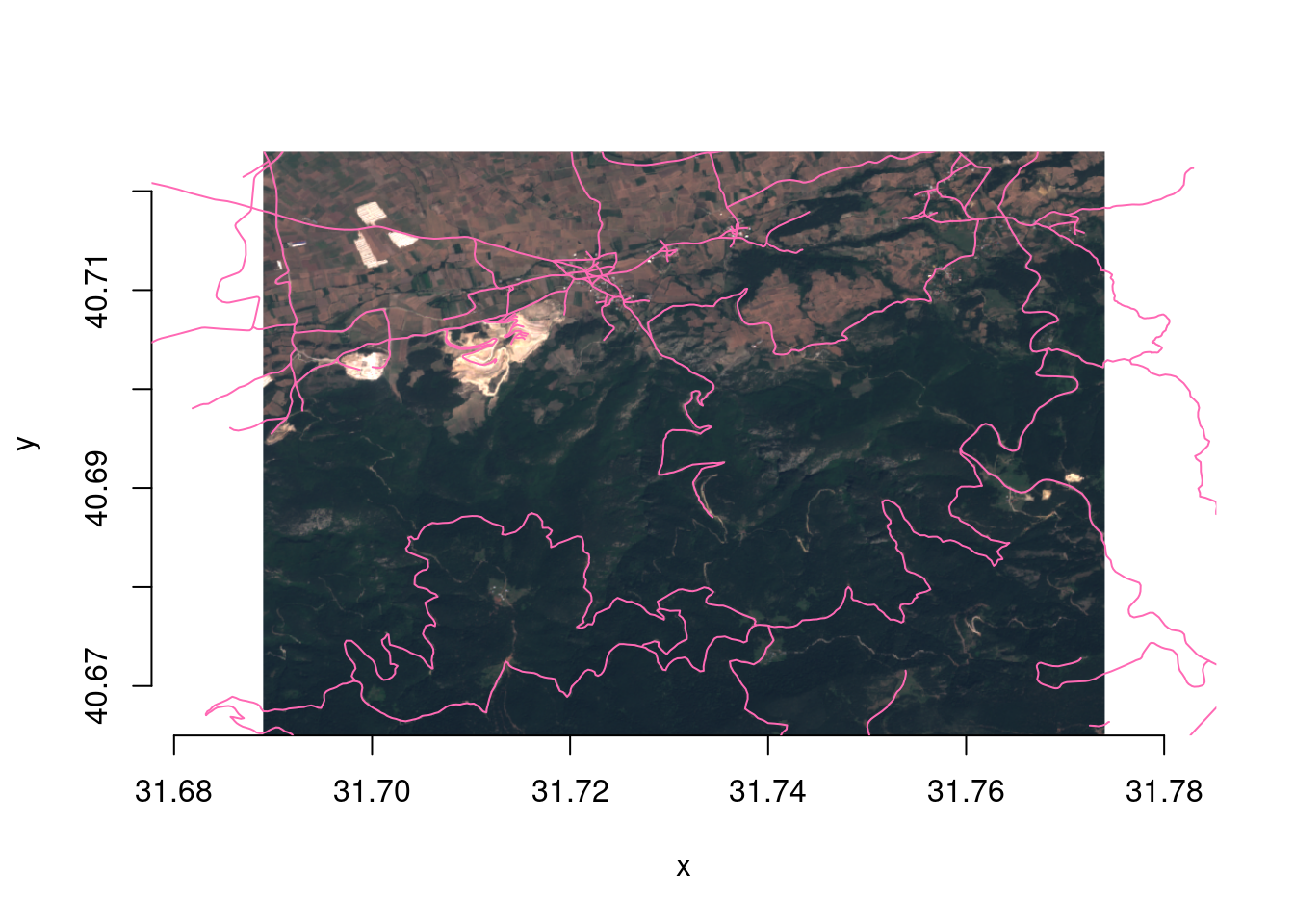
Summary
We had a look at GDAL multidimensional API, converting a 3D dataset to classic raster, augmenting the missing CRS information on a virtual copy and then warping an image to a familiar map context.
There is ongoing work to bring the full GDAL API to R in {gdalraster}, and in-development version of gdalraster to add the GDALMultiDimRaster class and helpers: https://github.com/mdsumner/gdalraster/tree/multidimnew.
Please get in touch if any of this is of interest!
Late Bonus Section: Bluelink ocean model
This is something I want to use VRT to encapsulate as one whole dataset, here just a test on one file (there are 174 of these ocean_temp files, up to June 2024 at time of writing).
Note that we are using ‘/fileServer/’ from Thredds, not ‘/dodsC/’. GDAL uses userfaultd as a trick to read NetCDF remotely.
from osgeo import gdal
dsn = "/vsicurl/https://thredds.nci.org.au/thredds/fileServer/gb6/BRAN/BRAN2023/daily/ocean_temp_2010_01.nc"
ds = gdal.OpenEx(dsn, gdal.OF_MULTIDIM_RASTER)
rg = ds.GetRootGroup()
rg.GetMDArrayNames()
# ['xt_ocean', 'yt_ocean', 'st_ocean', 'Time', 'nv', 'st_edges_ocean', 'average_T1', 'average_T2', 'average_DT', 'Time_bnds', 'temp']

temp = rg.OpenMDArrayFromFullname("//temp")
[d.GetName() for d in temp.GetDimensions()]
#['Time', 'st_ocean', 'yt_ocean', 'xt_ocean']
[d.GetSize() for d in temp.GetDimensions()]
#[31, 51, 1500, 3600]
I don’t know why xarray can seemingly read netcdf from S3, but not from normal url? Maybe just something fsspec I need to understand?
I also noticed that if the file is local the array names at root level are like this:
['//xt_ocean', '//yt_ocean', '//st_ocean', '//Time', '//nv', '//st_edges_ocean', '//average_T1', '//average_T2', '//average_DT', '//Time_bnds', '//temp']
gdalraster::gdal_version()[1] "GDAL 3.11.0dev-dd6009a0eb, released 2018/99/99"
[2] "3110000"
[3] "20189999"
[4] "3.11.0dev-dd6009a0eb" devtools::session_info()─ Session info ───────────────────────────────────────────────────────────────
setting value
version R version 4.4.2 (2024-10-31)
os Ubuntu 20.04.6 LTS
system x86_64, linux-gnu
ui X11
language (EN)
collate en_AU.UTF-8
ctype en_AU.UTF-8
tz Australia/Hobart
date 2025-03-12
pandoc 3.2 @ /usr/lib/rstudio-server/bin/quarto/bin/tools/x86_64/ (via rmarkdown)
─ Packages ───────────────────────────────────────────────────────────────────
package * version date (UTC) lib source
bit 4.5.0.1 2024-12-03 [2] CRAN (R 4.4.2)
bit64 4.6.0-1 2025-01-16 [2] CRAN (R 4.4.2)
cachem 1.1.0 2024-05-16 [2] CRAN (R 4.4.1)
class 7.3-23 2025-01-01 [4] CRAN (R 4.4.2)
classInt 0.4-11 2025-01-08 [2] CRAN (R 4.4.2)
cli 3.6.4 2025-02-13 [2] CRAN (R 4.4.2)
codetools 0.2-20 2024-03-31 [4] CRAN (R 4.4.1)
curl 6.2.1 2025-02-19 [2] CRAN (R 4.4.2)
DBI 1.2.3 2024-06-02 [2] CRAN (R 4.4.1)
devtools 2.4.5 2022-10-11 [2] CRAN (R 4.4.1)
digest 0.6.37 2024-08-19 [2] CRAN (R 4.4.1)
e1071 1.7-16 2024-09-16 [2] CRAN (R 4.4.1)
ellipsis 0.3.2 2021-04-29 [2] CRAN (R 4.4.1)
evaluate 1.0.3 2025-01-10 [2] CRAN (R 4.4.2)
fastmap 1.2.0 2024-05-15 [2] CRAN (R 4.4.1)
fs 1.6.5.9000 2024-12-18 [2] Github (r-lib/fs@8d40528)
gdalraster * 1.12.0.9250 2025-03-10 [1] local
generics 0.1.3 2022-07-05 [2] CRAN (R 4.4.1)
glue 1.8.0 2024-09-30 [2] CRAN (R 4.4.1)
here 1.0.1 2020-12-13 [2] CRAN (R 4.4.1)
htmltools 0.5.8.1 2024-04-04 [2] CRAN (R 4.4.1)
htmlwidgets 1.6.4 2023-12-06 [2] CRAN (R 4.4.1)
httpuv 1.6.15 2024-03-26 [2] CRAN (R 4.4.1)
httr2 1.1.0 2025-01-18 [2] CRAN (R 4.4.2)
jsonlite 1.9.0 2025-02-19 [2] CRAN (R 4.4.2)
KernSmooth 2.23-26 2025-01-01 [4] CRAN (R 4.4.2)
knitr 1.49 2024-11-08 [2] CRAN (R 4.4.2)
later 1.3.2 2023-12-06 [2] CRAN (R 4.4.1)
lattice 0.22-6 2024-03-20 [4] CRAN (R 4.4.1)
lifecycle 1.0.4 2023-11-07 [2] CRAN (R 4.4.1)
lubridate 1.9.4 2024-12-08 [2] CRAN (R 4.4.2)
magrittr 2.0.3 2022-03-30 [2] CRAN (R 4.4.1)
Matrix 1.7-0 2024-04-26 [2] CRAN (R 4.4.1)
memoise 2.0.1 2021-11-26 [2] CRAN (R 4.4.1)
mime 0.12 2021-09-28 [2] CRAN (R 4.4.1)
miniUI 0.1.1.1 2018-05-18 [2] CRAN (R 4.4.1)
nanoarrow 0.6.0 2024-10-13 [2] CRAN (R 4.4.2)
osmdata * 0.2.5 2023-08-14 [2] CRAN (R 4.4.2)
pkgbuild 1.4.4 2024-03-17 [2] CRAN (R 4.4.1)
pkgload 1.4.0 2024-06-28 [2] CRAN (R 4.4.1)
png 0.1-8 2022-11-29 [2] CRAN (R 4.4.1)
profvis 0.4.0 2024-09-20 [2] CRAN (R 4.4.1)
promises 1.3.0 2024-04-05 [2] CRAN (R 4.4.1)
proxy 0.4-27 2022-06-09 [2] CRAN (R 4.4.1)
purrr 1.0.4.9000 2025-02-19 [2] Github (tidyverse/purrr@9c8beb4)
R6 2.6.1 2025-02-15 [2] CRAN (R 4.4.2)
rappdirs 0.3.3 2021-01-31 [2] CRAN (R 4.4.1)
Rcpp 1.0.14 2025-01-12 [2] CRAN (R 4.4.2)
remotes 2.5.0 2024-03-17 [2] CRAN (R 4.4.1)
reticulate * 1.41.0 2025-02-24 [2] CRAN (R 4.4.2)
rlang 1.1.5 2025-01-17 [2] CRAN (R 4.4.2)
rmarkdown 2.29 2024-11-04 [2] CRAN (R 4.4.2)
rprojroot 2.0.4 2023-11-05 [2] CRAN (R 4.4.1)
rstudioapi 0.16.0 2024-03-24 [2] CRAN (R 4.4.1)
sessioninfo 1.2.2 2021-12-06 [2] CRAN (R 4.4.1)
sf * 1.0-19 2024-11-05 [2] CRAN (R 4.4.2)
shiny 1.9.1 2024-08-01 [2] CRAN (R 4.4.1)
timechange 0.3.0 2024-01-18 [2] CRAN (R 4.4.1)
units 0.8-5 2023-11-28 [2] CRAN (R 4.4.1)
urlchecker 1.0.1 2021-11-30 [2] CRAN (R 4.4.1)
usethis 3.0.0 2024-07-29 [2] CRAN (R 4.4.1)
vctrs 0.6.5 2023-12-01 [2] CRAN (R 4.4.1)
withr 3.0.2 2024-10-28 [2] CRAN (R 4.4.1)
wk 0.9.4 2024-10-11 [2] CRAN (R 4.4.1)
xfun 0.50 2025-01-07 [2] CRAN (R 4.4.2)
xml2 1.3.6 2023-12-04 [2] CRAN (R 4.4.1)
xtable 1.8-4 2019-04-21 [2] CRAN (R 4.4.1)
yaml 2.3.10 2024-07-26 [2] CRAN (R 4.4.1)
[1] /perm_storage/home/mdsumner/R/x86_64-pc-linux-gnu-library/4.4
[2] /usr/local/lib/R/site-library
[3] /usr/lib/R/site-library
[4] /usr/lib/R/library
─ Python configuration ───────────────────────────────────────────────────────
python: /perm_storage/home/mdsumner/.cache/R/reticulate/uv/cache/archive-v0/twFzciVwGCsaiQXG6_cWf/bin/python3
libpython: /perm_storage/home/mdsumner/.local/share/uv/python/cpython-3.11.11-linux-x86_64-gnu/lib/libpython3.11.so
pythonhome: /perm_storage/home/mdsumner/.cache/R/reticulate/uv/cache/archive-v0/twFzciVwGCsaiQXG6_cWf:/perm_storage/home/mdsumner/.cache/R/reticulate/uv/cache/archive-v0/twFzciVwGCsaiQXG6_cWf
virtualenv: /perm_storage/home/mdsumner/.cache/R/reticulate/uv/cache/archive-v0/twFzciVwGCsaiQXG6_cWf/bin/activate_this.py
version: 3.11.11 (main, Feb 12 2025, 14:51:05) [Clang 19.1.6 ]
numpy: /perm_storage/home/mdsumner/.cache/R/reticulate/uv/cache/archive-v0/twFzciVwGCsaiQXG6_cWf/lib/python3.11/site-packages/numpy
numpy_version: 2.2.3
osgeo: /perm_storage/home/mdsumner/.cache/R/reticulate/uv/cache/archive-v0/twFzciVwGCsaiQXG6_cWf/lib/python3.11/site-packages/osgeo
NOTE: Python version was forced by py_require()
──────────────────────────────────────────────────────────────────────────────reticulate::py_require()══════════════════════════ Python requirements ══════════════════════════── Current requirements ───────────────────────────────────────────────── Python: [No Python version specified. Will default to '3.11.11']
Packages: numpy, gdal── R package requests ───────────────────────────────────────────────────R package Python packages Python version
reticulate numpy